by James A. Marusek
February 9, 2018
from WattsupWithThat Website
 

I. Introduction

The sun is the natural source of heat and light for our planet.

Without our sun, the earth would be a cold dead planet adrift in space. But the sun is not constant. It changes and these subtle changes affect the Earth's climate and weather.

At the end of solar cycle 23, sunspot activity declined to a level not seen since the year 1913. [Comparing Yearly Mean Total Sunspot Numbers] ¹

The following was observed during the solar cycle 24:

1. The number of sunspots over the entire solar cycle decreased significantly by 50% or greater.
    

2. There were fewer solar flares and coronal mass ejections (CME's), which produces Solar Proton Events (SPE's) and geomagnetic storms on Earth.

    

   During the transition, beginning in July 2000, the sun produced 6 massive explosions in rapid succession. Each of these explosions produced solar proton events with a proton flux greater than 10,000 pfu @ >10 MeV.

    

   These occurred in July 2000, November 2000, September 2001, two in November 2001, and a final one in October 2003. And there hasn't been any of this magnitude since. ²
    

3. The magnetic field exerted by the sun significantly weakened.

    

   The Average Magnetic Planetary Index (Ap index) is a proxy measurement for the intensity of solar magnetic activity as it alters the geomagnetic field on Earth. It has been referred to as the common yardstick for solar magnetic activity.

    

   Ap index measurements began in January 1932. The quieter the sun is magnetically, the smaller the Ap index. During the 822 months between January 1932 and June 2000, only one month had an average Ap index that dropped down to 4.

    

   But during the 186 months between July 2000 and December 2015, the monthly Ap index fell to 4 or lower on 15 occasions. ³
    

4. The number of Galactic Cosmic Rays (GCRs) striking Earth increased. GCRs are high-energy charged particles that originate outside our solar system. They are produced when a star exhausts its nuclear fuel and explodes into a supernova.

    

   The Sun's magnetic field modulates the GCR flux rate on Earth.

    

   Cosmic rays are deflected by the interplanetary magnetic field embedded in the solar wind, and therefore have difficulty reaching the inner solar system. The effects from the solar winds are felt at distance approximately 200 AU from the sun, in a region of space known as the Heliosphere.

    

   As the sun went quiet magnetically, the Heliosphere shrunk, and a greater number of these particles penetrated into the Earth's atmosphere. The sun's interplanetary magnetic field fell to around 4 nano-Tesla (nT) from a typical value of 6 to 8 nT. The solar wind pressure went down to a 50-year low.

    

   The heliospheric current sheet flattened. In 2009, cosmic ray intensities increased 19% beyond anything that was seen since satellite measurements began 50 years before. ⁴
    

5. In general, the sun's total irradiance varies about 0.1 percent over normal solar cycles.

    

   But this variation is not linear across the entire radiation spectrum. Between 2004 and 2007, it was observed that the decrease in ultraviolet radiation (with wavelengths of 400 nanometers) was 4 to 6 times larger than expected, whereas the visible light (400-700 nanometers) showed a slight increase. ⁵

    

   This is significant because Solar UV flux is a major driver of stratospheric chemistry.
    

6. The upper atmosphere of Earth collapsed.

    

   The thermosphere ranges in altitude from 90 km to 600+ km above the Earth's surface. During the depth of last solar minimum in 2008-2009, the thermosphere contracted by the largest amount observed in at least the last 43 years.

    

   The magnitude of the collapse was two to three times greater than low solar activity could explain. ⁶
    

7. Solar radio flux during the peak of the solar cycle diminished significantly.

    

   The F10.7 index is a measure of the solar radio flux per unit frequency at a wavelength of 10.7 cm, near the peak of the observed solar radio emission.

    

   The solar cycle minimum produced the lowest F10.7 flux since recordings began in February 1947. ⁷
    

8. Sightings of noctilucent clouds (or night clouds) are appearing at lower latitudes.

    

   These clouds are formed from ice crystals in the extreme upper atmosphere, called the mesosphere. Noctilucent clouds (NLCs) were first reported by Europeans in the late 1800s.

    

   In those days, you had to travel to latitudes well above 50º to see them.

    

   Now, however, NLCs are spreading. In recent years they have been sighted as far south as Colorado and Utah in the United States.

II. Background - Solar Cycles

Sunspots are dark spots that appear on the surface of the sun. They are the location of intense magnetic activity and they are the sites of very violent explosions that produce solar storms.

The sun goes through a cycle lasting approximately 11 years.

It starts at a solar minimum when there are very few sunspots and builds to a solar maximum when hundreds of sunspots are present on the surface of the sun and then returns back to a solar quiet minimum.

This cycle is called a solar cycle. We are currently in the solar minimum separating Solar Cycle 24 and 25.

The first solar cycle documented by scientist began in March 1755.
 

Figure 1.

Image of Solar Cycle 23 from the

Solar and Heliospheric Observatory

(SOHO) by Steele Hill (NASA GSFC)
 

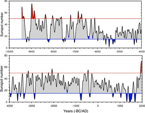
Figure 2.

Sunspot activity throughout the Holocene.

Blue and red areas denote grand minima and maxima, respectively.

The entire series is spread out over two panels

for better visibility. ref8

The sun exhibits great variability in the strength of each solar cycle.

Some solar cycles produce a high number of sunspots. Other solar cycles produce low numbers. When a group of cycles occur together with high number of sunspots, this is referred to as a solar Grand Maxima.

When a group of cycles occur with minimal sunspots, this is referred to as a solar Grand Minima. Usoskin details the reconstruction of solar activity during the Holocene period from 10,000 B.C. to the present. ⁸

Refer to Figure 2.

• The red areas on the graph denote energetic solar Grand Maxima states.

• The blue areas denote quiet solar Grand Minima states.

The reconstructions indicate that the overall level of solar activity observed in the middle of the 20^th century stands amongst the highest of the past 10,000 years.

The 20^th century produced a very strong solar Grand Maxima.

Typically these Grand Maxima's are short-lived lasting in the order of 50 years. The reconstruction also reveals Grand Minima epochs of suppressed activity, of varying durations have occurred repeatedly over that time span.

A solar Grand Minima is defined as a period when the (smoothed) sunspot number is less than 15 during at least two consecutive decades.

The sun spends about 17 percent of the time in a Grand Minima state.

Examples of recent extremely quiet solar Grand Minima are the,

• Maunder Minimum (about 1645-1715 A.D.)

• Spörer Minimum (about 1420-1570 A.D.)

The sun has undergoing a state change. It transitioned from a Grand Solar Maxima, which typified the 20^th century to a magnetically quiet solar period similar to a Dalton Minimum.
 

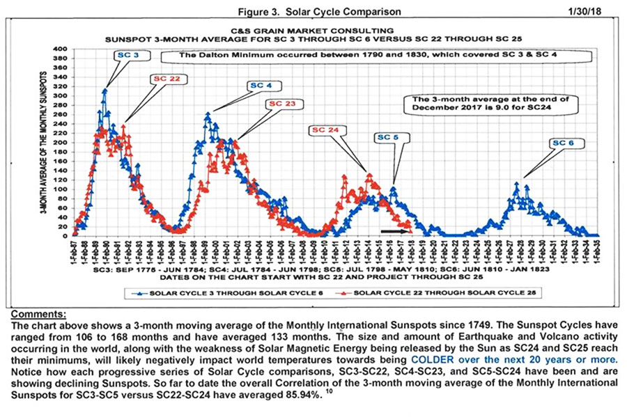
III. Detailed Forecast

I predict that the intensity of Solar Cycle 25 will be fairly similar to Solar Cycle 24.

I base this prediction on two observations:

1. The pattern seen in Solar Cycles 22 through 25 matches fairly close to the historical pattern seen in Solar Cycles 3 through 6. Refer to Figure 3.

    

   Solar Cycle 4 to Solar Cycle 7 corresponded to a period known as the Dalton Minimum.

    

   The Dalton Minimum was a time of minimal sunspots, a series of weak solar cycles; but it is not weak enough to be described as a Solar Grand Minima.
    

2. Solar cycles come in pairs.

    

   A solar cycle is in reality a half cycle. It takes two solar cycles to complete one full cycle. In one solar cycle, the magnetic polarity of the sun faces north and in the next it faces south.

    

   At the end of 2 solar cycles the sun is back to its original starting point. So they are two different sides of the same coin. The intensity of each half cycle is approximately equal.

In my opinion, the most interesting part of the upcoming solar cycle is the period of minimal sunspots ^Å rather than the period of maximum sunspots because the minimum represents the extreme, the primary actor that foreshadows weather events.

When I compared this upcoming period of minimal sunspots with the corresponding period of minimal sunspots during the Dalton Minimum (between solar cycle 5 and 6), I made the following predictive observation.

The upcoming period of minimal sunspots will extend from the winter of 2016/17 to the winter of 2024/25. This period is analogous to the similar Dalton Minimum timeframe from the winter of 1806/07 to the winter of 1814/15.

I predict this upcoming period of minimal sunspots shall be longer and deeper than the last one. The changes during this solar minimum shall be more pronounced than during the last solar minimum.

These parameters include,

• sunspot numbers

• Average Magnetic Planetary Index (Ap index)

• Galactic Cosmic Rays (GCRs) flux rates

• heliosphere volume

• the sun's interplanetary magnetic field strength

• solar wind pressure

• solar Ultra Violet (UV) flux rate

• Earth's thermosphere volume

• solar radio flux per unit frequency at a wavelength of 10.7 cm

• the latitude of Noctilucent Clouds (NLC) sightings

Early scientist have associated the weakest solar cycles that occur in Solar Grand Minima events such as the Wolf Minimum, Spörer Minimum and Maunder Minimum with periods of extreme cold, the Little Ice Age.

The theories that sunspots intensity correlates to Earth's climate and weather changes was a predominant mainstream theory that goes back centuries. In 1801, the great astronomer William Herschel observed a correlation between sunspots and wheat yields in England. Periods of minimal sunspots produced adverse growing seasons that produced minimal crop yields.

In 1873, a Russian-German climatologist Wladmir Peter Köppen, using temperature data collected from 403 stations over the whole earth concluded that the maximum temperatures observed in the tropics corresponded to sunspot minimums.

In 1891, Henry F. Blanford published a series of temperature measurements taken by Professor S.A. Hill with the solar thermometer that is black bulb and vacuum thermometer, for the years 1875 to 1885 at Allahabad (25.4°N latitude) that showed an annual mean temperature difference of 3.7°C (6.6°F) between sunspot minimum and sunspot maximum.

In 1872, Scottish meteorologist and astronomer Charles Meldrum, showed that periods of minimal sunspots also corresponded to periods of minimal rainfall at tropical weather stations.

Sir Norman Lockyer showed this was also the case for several meteorological stations in Ceylon and in India. ⁹

But this relationship does not affect the entire globe equally.

The research by,

• Charles Chambers (1857)

• Frederick Chambers (1878)

• S.A. Hill (1879)

• E.D. Archibald (1879)

• Henry F. Blanford (1879, 1880),

...provided interesting findings.

• In low latitudes, the barometric pressure is higher during periods of low sunspots (solar minimums).

   

• But in mid latitudes, the barometric pressure is exactly opposite; it is higher during solar maximums in the winter.

   

• And in polar latitudes, the barometric pressure is higher during the solar minimums during the summer. ⁹

Great storms with high winds generally occur when high-pressure regions clash with low-pressure regions.

In 1891, H.F. Blanford noted that during solar sunspot minimum a smaller portion of the tropical atmosphere is transferred to high latitudes in the winter hemisphere. ⁴⁷ In the temperate zones the sunspot frequency appeared to be related to the approach of very cold winter.

 

In mid latitude regions at Greenwich, England, Alexander B. MacDowall analyzed the data for the period October to March for the year 1841-1895. Low sunspot frequency corresponded to an increase in the number of days with a (cold) north wind. ⁴⁸ The number of days of frost [days when temperature fell below 32°F] in London also correlates to periods of minimal sunspots. ⁹

 

H. Helm Clayton in 1895 found a very similar correlation between days of frost and periods of minimal sunspots at both Paris, France and in New England. But in his case, he based his findings on the full (22 year) cycle rather than the half (11 year) solar cycle. ⁵⁵

Björn Helland-Hansen and Dr. Fridtjof Nansen found a similar correlation at the Lighthouse on Ona Island, Norway (Latitude 62.9°N). They compared the mean winter air temperature from 1 November to April 30 for the years 1875-1907 and showed that colder temperatures generally occurred during periods of minimal sunspots. ⁵⁶

Many times the data analyzing a linkage between climate and solar cycle appeared to be conflicted or contradictory.

I feel this was due primarily to the data being sifted through the wrong filters. By its very nature weather is a chaotic system. I also feel that as the period of minimal sunspots became shorter and less extreme, especially during the Grand Solar Maxima that typified the 20^th century, the observational trends became less pronounced.

Several early scientists including,

• Sir (Joseph) Norman Lockyer (professor of Astronomical Physics and the founding editor of the journal Nature)

• William James Stewart Lockyer

• American Professor F. H. Bigelow

• Dr. Major Albert Veeder M.D.

• American professor C.J. Kullmer

• Norwegian professor Björn Helland-Hansen

• Dr. Fridtjof Nansen [the Arctic explorer],

...and others believed that the climate variations on Earth due to changes in solar sunspot activity is primarily driven by Earth's atmospheric circulation rather than by being driven by the effects of direct solar heating. ¹¹

The scientific underpinnings that explain these correlation was lacking in historical times.

It is only in modern times that scientist have been able to measure the various important solar, space and earth metrics and evolve theories to explain this correlation.

In 2016, I authored a paper titled Little Ice Age Theory in an attempt to provide those details and relationships. ¹²

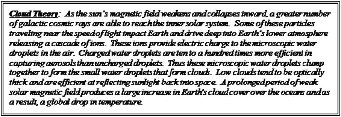
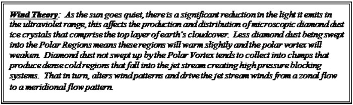
In that paper, I identified two main theories called Cloud Theory and Wind Theory.

Cloud theory describes a long-term climate driver whereas wind theory describes a shorter-term weather driver.

Both these theories revolve around the solar interaction on Earth's cloud formation.

• The cloud theory deals with the ability of low-level clouds to slowly alter temperature.

   

• The wind theory deals with the ability of high-level clouds to alter atmospheric circulation.

I predict that this upcoming solar minimum will produce an increase in ocean cloud cover and a gradual drop in global temperatures.

The global warming pause or hiatus will continue. (According to the most accurate temperature data from satellites, global temperatures flatlined after 1998.) ¹³

Cloud theory primarily impacts Earth's long-term climate.

When the Solar Grand Minima (Spörer Minimum and Maunder Minimum) came to an end, the extreme cold did not change overnight. Rather, the change was gradual, taking many decades for the Earth to warm up.

By the same token, when the Solar Grand Maxima that typifies the 20^th century warm period came to an abrupt end, the Earth will not slide into another little ice age overnight.

This is due to the latent heat stored in the Earth's landmass and oceans.

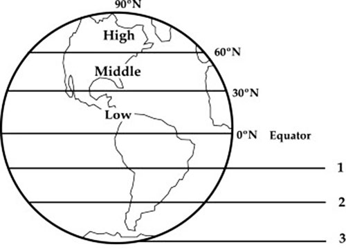
During the winter in the Northern Hemisphere, a meridional jet stream flow pattern will pull frigid arctic air from the North deep into mid latitude [30°and 60°N] regions.

This will produce record snowfalls and record lows. The extreme cold can freeze rivers and lakes. The meridional jet stream will produce very violent winter storms and these storms will have explosive energy - strong winds. At the end of winter, great floods called freshets can occur.

Extreme winters can shorten the crop-growing season producing scarcity and famines.

The historical term freshet is most commonly used to describe a spring thaw resulting from snow and ice melt in rivers located in the northern latitudes.

A freshet generally occurs when either the ground is frozen or when it is so saturated by moisture from the spring thaw, that any additional moisture will simply be runoff.

At that time if the depth of the snowfall was deep during the winter and the melt off very rapid, or if heavy rainfalls strike the area, great floods can occur.

When the ice in rivers and lakes break up, the chunks of ice can flows downstream and can create ice dams. Generally these occur at bends of a river or other obstructions in the river such as arches of bridges, or weirs.

When this occurs, the swollen rivers can overflow many riverbanks causing great destruction to cities and farmland.

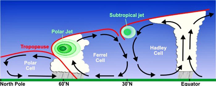
Figure 4

Jet Stream in Northern Hemisphere
 

The two jet streams (Polar and Subtropical Jet Streams) are interlocked together.

When the polar jet changes from a zonal to meridional flow pattern, it will also affect the subtropical jet that pulls moisture from the equator and will weakens the trade winds.

This will affects the major flood cycles in the Northern Hemisphere such as the Nile River inundation, and the India monsoons for which much of the world depends on food.

So whereas,

• scarcity and famines in the Ferrel Cell [30°to 60°N] can be caused by shorter growing seasons, freshets and erratic weather patterns

   

• famines in the northern Hadley Cell [0°to 30°N] can be caused by major droughts

The same process occurs in the Southern Hemisphere but the Earth's atmospheric circulation pattern is not symmetrical.

This is due to the distribution of landmasses, especially the tall mountain ranges. As a result in the Southern Hemisphere winter the polar vortex is generally located between 50°and 65°S latitude, whereas in the Northern Hemisphere the polar vortex is located between 30°and 60°N latitude.

Therefore the location of the Hadley Cell and Ferrel Cell cover different asymmetrical latitude ranges within each hemisphere.

In the mid-latitude regions, I forecast the period of minimal sunspots preceding solar cycle 25 will be responsible for,

• record low temperatures during the winter

• record snowfalls

• powerful and energetic winter storms

• frozen lakes and rivers

• great spring floods (freshets)

• weather induced famines/scarcities due to shortened growing seasons, freshets and erratic weather patterns

In the low-latitude regions, I forecast the period of minimal sunspots preceding solar cycle 25 will be responsible for,

• lower rainfall, higher temperatures and droughts

• weather induced famines/scarcities due to droughts

Source

Any meteorological theory describing weather and climate should be grounded in a firm knowledge and understanding of the past.

For this reason, I have included in the next section a listing of weather events that document the analogous timeframe within the Dalton Minimum.

The solar minimum period from the winter of 1806/07 to the winter of 1814/15 should be similar to the period from the winter of 2016/17 to the winter of 2024/25.

IV. Analogous Period
Weather Events between the Winters of 1806/07 and 1814/15 that can be attributed to a Weak Solar Minimum
 

Great Britain 1809 & 1810

Extreme solar minimums can produce record cold temperatures, record snowfalls, fierce winter storms, frozen lakes & rivers, and spring floods (freshets) within the Ferrel Cell [30°N to 60°N]. Sometimes many elements can conspire together to create great disasters.

In January 1809, an extreme cold spell struck England and the ground froze solid. This was followed by several days of heavy snowfall. The snow accumulations were up to three feet deep (91 centimeters) and "no doubt more over upland areas".

 

Then beginning around 24 January, the temperature rose suddenly and heavy rains fell across the nation. All the snow melted suddenly and since the ground was frozen, the rainwater and snowmelt produced a great flood (freshet). ¹⁴

"Almost every river in the Kingdom has overflowed its banks and immense tracts of land have been under water." ¹⁵

Prior to the thaw many roofs were covered with snow. Snow acts like a sponge and absorbs rainwater.

 

The weight of the rain soaked snow placed a heavy weight load on the roofs and as a result many roofs collapsed.

"In Lambeth all the lower apartments of some hundreds of houses are three and four feet under water; and throughout the metropolis, and its neighborhood, few houses have escaped a drenching from top to bottom, excepting those from the roofs of which the inhabitants took the precaution to have the snow removed previous to the commencement of the thaw." ¹⁴

"Water flowing through cellars, shops and ground floors of building, so that goods were washed away or made worthless, and inhabitants had to retreat upstairs and be supplied with food and fuel through windows from boats and carts.

 

Work was disrupted, streets were filled with torrents carrying away all manner of debris, building had to be abandoned, or they collapsed killing or injuring their occupants. Many people lost their all and were totally ruined."

 

"Travel was impossible on foot and could be dangerous for carts and carriages"

 

"In the countryside, vast areas were inundated, and livestock were drowned before their owners could get them to higher ground.

 

Barns were flooded, and wagons, field gates, fences and hay ricks were carried away.

 

Coach services were interrupted and mail was got through by using circuitous routes; carters misjudging the depth of water on the road lost their horses and farmers had their crops destroyed. Along the river, traffic was delayed, barges sunk, mills stopped working and weirs were damaged.

 

In many places this was the worst flood for decades or 'beyond the memory of man'." ¹⁴

The swollen rivers overflowed many riverbanks.

 

One of the hazards from a freshet is caused by the ice from frozen rivers. When the ice breaks up, it flows downstream and can create ice dams.

 

Generally these occur at bends of a river or other obstructions in the river such as arches of bridges, or weirs [A weir is a barrier across the horizontal width of a river that alters the flow characteristics of the water and usually results in a change in the height of the river level].

 

In this flood,

"About a mile above Carlisle, the weir that diverts the Calder to Messrs Losh & Co.'s print work flowed into the adjoining grounds… and swept away large trees of various kinds.

 

The river having now lost its natural channel, the new one produced the most dreadful ravages in its progress." ¹⁴

Many large cities contain rivers. Ice dams can break up very suddenly and send a wall of water downstream causing great damage.

This freshet, which extended widely across much of England but to a lesser degree in Wales and Scotland, also destroyed or damaged many bridges. This flood collapsed the bridge at Wallingford over the river Thames.

 

Part of the old bridge over the river Thames at Wheatley near Oxford gave way. The bridge between Pangbourne and Whitchurch was very severely damaged.

 

Also the bridges at Twyford, on the London road from Reading were broken down. In Devon the Feniton bridge over the river Otter gave way.

 

Also in Devon,

"the center arch on the main river Exe at Cowley-bridge fell in and the Bickleigh-bridge was so damaged to render the road to Tiverton impassable".

In Wales, the bridge over the river Usk at Crickhowell was carried away. In Scotland, the bridge over the river Yarrow, two miles from Selkirk was entirely swept away.

 

The Inchinnan Bridge over the Black Cart Water near Paisley collapsed in the flood. ¹⁴

The harvest weather of 1809 [from July to October] was exceedingly wet. Large portions of the wheat suffered from mildew and from sprouting. ¹⁶

 

During the next winter a great storm struck England in December.

 

A great deal of snow fell in the interior of the country. It is said to be lying in drifts of nine feet deep in some places on the east side of the country and the adjoining part of Northumberland. ¹⁷

 

From 13 January 1810 to March the Midlands of England experienced freezing conditions with snow and hard frost affecting the young crops. The month of May brought in night frosts. ¹⁵

 

In 1810, England imported over a half a million tons of wheat, flour, other grains and meal.

"But for that importation, it would have been a year of famine." ¹⁶

 

Mississippi River

In four years out of this eight-year period, the Mississippi River in the United States experienced major floods or one might even say great floods.

 

These were years 1809, 1811, 1813, and 1815. The flood of 1815 was due to freshets in the Ohio River, the Upper Mississippi River, the Missouri River, the Cumberland River and the Tennessee River. ¹⁸

In the flood of 1813, the Mississippi River overflowed its banks and flooded the country on the west side inundating it to the distance of 65 miles, by which 22,000 head of cattle were destroyed. ¹⁹

The flood of 1809, inundated all the plantations near Natchez, Mississippi and the flood destroyed the crops. ¹⁸
 

 

Winter of 1806/07

The winter of 1806/07 in the U.S. was long, and produced extreme cold, great snowfalls and several freshets.

In Philadelphia, Pennsylvania, the first frost occurred on 17 October 1806. And there were deep snows from the 4^th to the 12^th of December. ²⁰

On 26 January 1807, an extreme cold spell struck New England.

 

On that day temperatures fell to,

• -13º F in Cambridge, Massachusetts

• -33º F at Hollowell in Kennebec County, Maine

• -9º F at Portsmouth, New Hampshire

• -4º F at Boston, Massachusetts

• -12º F at Smithfield, Rhode Island

• -6º F at Hartford, Rhode Island

• -15º F at Warwick, Massachusetts

• -10º F at Deerfield, Massachusetts ²¹

On 9 February 1807 and another cold spell struck which dropped temperatures at Deerfield, Massachusetts to -14º F and at Albany, Vermont down to -20º F. ²¹

A great flood struck New England in the United States during the beginning of February 1807.

 

The freshet was caused by heavy rains, which melted the snow and swelled the rivers until they overflowed, carrying away bridges and mills, entering warehouses and stores and doing great damage.

 

The floods carried away several bridges east of Portsmouth, New Hampshire. It also took out a bridge over the Little River in Haverhill, Massachusetts. The principal bridge at Lawrence [connecting Andover and Methuen] was destroyed.

 

Other bridges further up the Merrimack River were destroyed. The Watertown Bridge and the Milford Bridge were carried away. At Pawtucket, Rhode Island, the bridge was destroyed along with a cotton factory and four or five other buildings.

 

In Connecticut, the stone bridge over Swallow-Tail Brook at East Chelsea was destroyed. The Shetucket River rose from 18 to 20 feet [5.5-6.1 meters].

 

At Norwich, Connecticut, the Lord and Lathrop bridges were swept away. The Lovett, Geometry and Quarter bridges were damaged. Water rose in houses compelling the inhabitants to climb out of their windows and be evacuated by boats. ¹⁹

 

Ice that floated down Deerfield river in Massachusetts during the flood in February 1807 was observed to be 2 feet 9 inches (84 centimeters) in thickness and the ground was frozen solid to a depth of 3 feet (91 centimeters). ²²

In the Midwest and South, 7 February 1807 was known for many years as "Cold Friday" by reason of the extreme low temperatures reached during that day. ^19,23

 

In Kentucky, temperatures dropped 60º F (33º C) within 12 hours. The violent snowstorm produced 6 inches of snowfall in Kentucky and bitter cold temperatures. ²⁴

In the United States a massive late-season snowstorm traveled from the Tennessee Valley to southeastern Pennsylvania on March 30-April 1, 1807.

 

At the western end in Vincennes, Indiana; snow fell to a depth of 11 inches.

 

The depth of the heavy wet snow in Pennsylvania was 36 inches (91 centimeters) at Huntingdon; 36-42 inches (91-107 centimeters) in the Nittany Valley; and 54 inches (137 centimeters) in Montrose.

 

In Bradford County, Pennsylvania near the New York border,

"snow fell continuously three days and was between four and five feet (1.2-1.5 meters) deep".

Snow fell to a depth of,

• 54 inches (137 centimeters) in Utica, New York

• 52 inches (132 centimeters) in Lunenburg, Vermont

• 60 inches (152 centimeters) at Danville, Vermont

• 48 inches (122 centimeters) at Montpelier, Vermont

• 42-48 inches (107-122 centimeters) at Norfolk, Connecticut ^19,25

In April, following the rapid thaw of this snow, one of the most notable floods of the Susquehanna River took place. On the last day in April, there was a very high freshet on the Connecticut River.

 

There was a great flood in May in the Monongahela river, forty feet above the common level at Brownsville, Pennsylvania that cause much damage. ^19,21,26
 

 

Frost Fairs

In Canada during the winter of 1807-1808, Lake Champlain, 120 miles in length, was frozen over and was crossed on the ice.

 

The Saint Lawrence River was frozen completely over, a few leagues above Quebec City and served as a road to Montreal. It seldom freezes over, opposite to Quebec City or in the basin because the river narrows at that spot, the currents are much stronger, and because the rising tides have such force that it keeps the floating masses of ice in constant motion.

 

During this winter it froze.

 

For a distance of eight miles, there was an immense sheet of ice, as smooth as a mirror. Thousands of people came on it daily. Booths were erected on the ice for their entertainment. Many people enjoyed skating on the ice.

 

Others drove across it in carrioles. [A carriole is a light small carriage, toboggan or sled drawn by a single horse.]

 

The ice was so thick that horses could travel on it safely. There were carriole races on the ice with great swiftness. It was a kind of jubilee, an ice fair. ²⁷

In England, on 27 December 1813, there was an impenetrable fog, which extended fifty miles round London, and continued for eight days. This fog was accompanied by a severe frost, which lasted six weeks.

 

On 14 January 1814, a tremendous fall of snow fell so deep in the West so as to impede traveling, and the severity of the intense cold was noticed in every part of England. And then the River Thames froze solid and became the site of the last great London frost fair.

 

During the whole week of 20 January, the River Thames below Windsor Bridge, called Mill River, had been frozen over, and was crowded with people skating.

 

The ice presented a most picturesque appearance. The view of St. Paul's and of the city, with the white foreground, had a very singular effect; in many parts large blocks of upheaved ice, resembled the rude interior of a stone quarry.

 

On 31 January a frost fair began to take shape.

 

On 3 February, large chalkboards were set up that read,

"A safe footway over the River to Bankside".

As a result thousands of people began to walk on the ice and to travel from the London Bridge to Blackfriars' Bridge, which became a grand mall or walk.

 

Many booths were erected in the very center of the river, formed from blankets and sailcloths, and ornamented with streamers and various signs. One of the tents exhibited a sheep roasting over an open fire.

 

In addition to,

"kitchen fires and furnaces… blazing and boiling in every direction, and animals, from a sheep to a rabbit, and a goose to a lark, were turning on numerous spits."

Many other activities were also underway.

 

Skittles, sledging [sledding], and bull-baiting were enjoyed, drinking tents were filled with people, and open fires had people sitting around drinking rum, grog, and other spirits. Tea, coffee, and eatables were also available.

 

There were also numerous booths selling toys, books, and trinkets labeled "Bought on the Thames."

 

Eight or ten printing presses were erected, and numerous pieces commemorative of the 'great frost' were printed on the ice. Even a dance was held. It was set up on a barge that had firmly frozen in place a considerable distance offshore. Thousands flocked to the spectacle.

 

Then around 5 February, the river began to break up and the last Great London Ice Fair came to an end. ^17,19,28
 

 

Famine in Ireland

The winter of 1813/1814 was very severe in Great Britain. It was remembered in many parts of England as the year of the "Great Frost".

"All over the country the mail coaches had to cease running, and in many instances were abandoned in the snow, the letters being sent on by the guards on horseback.

 

And even this means of conveyance proved unavailing in some localities, for when the snow lay four feet deep in the streets of the great towns, it may be fairly presumed that it proved a much more serious obstacle in the country." ²⁹

 

"The winter of 1813-1814 would eventually be considered 'one of the four or five coldest winters in the CET [Central England Temperature] record.'

 

The winter was also cold enough that the Thames became so solidly frozen someone dared take an elephant across it below the Blackfriars Bridge." ²⁸

On 11 January 1814, it was reported,

"The quantity of snow which has fallen in the upper part of Hampshire, and on the Hind Head is very great, lying in many places fifteen feet deep." ²⁷

On 13 January it was reported at Dublin, Ireland that there was an uncommon depth of snow and the streets appeared yesterday almost deserted. ¹⁷

 

At Nottinghamshire, England it was reported that after a dark, wet and cold start to spring, it remained very cold with some snow and sharp frosts through May, while June was also cold. ¹⁵

 

Just as in England, the winter was very severe in Ireland. The scarcity of food was severely felt by the Irish poor in 1814 in consequence of the failure of the potato crop. ¹⁹

 

The scarcity of the potato crop in Ireland in 1814 was due to the severity of the winter combined with a shortened growing season.
 

 

Extreme Cold

In the 16^th and 17^th centuries, European scientists invented a device that measured temperature called a thermometer.

 

Many of these early thermometers used alcohol or mercury (quicksilver). The thermometers were a sealed liquid-in-glass tube. A bulb at the bottom of the tube contained the liquid, which would expand with rising temperature.

 

These early thermometers used a variety of different scales such as Fahrenheit, Celsius and Réaumur among others. Mercury is a heavy, silvery-white liquid metal. It has a freezing point of -37.89°F (-38.83°C).

 

So in general, when the mercury froze in the thermometers it is indicative of extremely cold temperatures.

"From meteorological observations taken at Moscow [Russia], it appears that the greatest cold of last winter, was on the night of the 11th of January [1809].

 

Dr. Rehmann having exposed quicksilver to the open air in a cup, it froze so hard, that it could be cut with shears, and filed.

 

Count Boutourline found the mercury in three of his thermometers frozen, and withdrawn entirely into the ball; but in another thermometer, which was not frozen, from 6 in the morning of the 12th, till 35 minutes after, it was at 35º below 0 on the Réaumur [-43.8°F, -46.8°C]." ³⁰

Towards the end of March 1809, the mercury froze several times in the thermometer at Moscow, Russia and there was a great fall of snow. ^19,31

Quicksilver was frozen hard at Moscow, Russia on 13 January 1810. During a part of January 1810, the cold was so intense at Moscow, Russia that the mercury froze. ¹⁹

Alcohol based thermometers (spirit based thermometers) could measure colder temperatures than those that used mercury. Ethanol-filled thermometers are used in preference to mercury for meteorological measurements of minimum temperatures and can be used down to -94 °F (-70 °C).

During 1812 & 1813 the French army under Napoleon captured the burning and deserted city of Moscow, Russia and then retreated during one of Russia's harshest winters, the winter of 1812/13.

 

Winter took its grip over all of Europe at an early stage with severe cold. The first snow fell on Moscow on 13 October. The French army began to retreat on 18 October and completely evacuated the city by 23 October.

 

Under continuous snowfall the French army retreated to Smolensk, Russia. From 7 November onwards, extreme severe cold gripped the area. On 9 November, the thermometer dropped to -12°R. (5°F, -15°C).

 

Larrey [Dominique Jean Larrey, a French surgeon in Napoleon's army] carried a [Réaumur] thermometer [which used diluted alcohol] in the buttonhole of his tunic. [He kept a temperature record during the French retreat.]

 

The French army stayed at Smolensk from 14 to 17 November. As they left Smolensk, Larrey observed the temperature had dropped to -21°R. (-15.3°F, -26.3°C). The French Corps of Marshal Ney [that held the rear guard during the retreat] escaped [after being cut off by the Russian army] because on the night of 18/19 November, they crossed the frozen Dnieper River.

 

The night before a Russian army corps went with his artillery on the ice of the Dvina (Daugava) River.

 

On 24 November as Napoleon's troops approached the Berezina (Beresina) River the weather had turned warmer; the river began to thaw, and was impassable because of numerous ice floes [and bridges destroyed during the conflict]. This left the French army without a way to retreat, just as the Russian army was closing in.

 

On 26-29 November, the French hastily constructed temporary bridges and moved their troops across to the other side of the Berezina River. Immediately after, the cold began again with renewed intensity, the thermometer fell to -20°R. (-13°F, -25°C).

 

On 30 November it continued to decline to -24°R. (-22°F, -30°C). On 3 and 6 December at Molodechno (now Maladzyechna, Belarus) the temperature read -30°R. (-35.5°F, -37.5°C).

 

As this intense cold continued, the army continued its withdrawal to Vilna (now Vilnius, Lithuania). During the night of 9 December at Vilna, the temperature dropped to -32°R. (-40°F, -40°C).

 

On 11 and 12 December the French army crossed the ice of the Niemen River at Kovno (now Kaunas, Lithuania), and brought the few remaining remnants across the Vistula River and the Oder River to safety.

 

The Napoleon's army suffered more than 400,000 casualties during this campaign and much of this was due to the extreme cold and the lack of preparedness for the severe winter. ^19,32

At New Brunswick, Ontario, Canada, about midway between Moose Factory and Lake Superior, the lowest winter temperature in 1814 was -50°F (-45.6°C). ³³

M'Keevor wrote in his voyage to Hudson Bay in 1812 that,

"During the winter season, which usually continues for nine months, the spirit thermometer is commonly found to stand at [-]50. Quicksilver freezes into a solid mass…

 

Wine, and even ardent spirits, become converted into a spongy mass of ice; even the "living forest" do not escape, the very sap of the trees being frozen; which, owing to the internal expansion which takes place in consequence, occasionally burst with tremendous noise." ³⁴

 

"Cold Friday" Bomb Cyclone

The "Cold Friday" of 19 January 1810 was a lethal event because the great winds and the sudden, steep drop in temperature, which caught many people off guard.

 

At the coastal New England city of Boston, Massachusetts, the temperature dropped 57º F (31.7ºC) in less than 24 hours.

 

The coastal city of Portsmouth, New Hampshire experienced a 54º F drop. The ocean moderates temperatures and inland regions experienced greater extremes. In Cheshire County, New Hampshire, the temperature dropped

63º F within 12 hours. At Warren, New Hampshire the temperature fell from 43º F to -25º F in 16 hours, a temperature drop of 68°F. Several journals claimed the mercury dropped 100 degrees in less than 24 hours, from 67°F to -33°F.

 

During the daylong storm, the heavens roared like the sea in a cyclone.

 

Thousands of farmyard fowl were blown away and never seen again; rabbits, partridges and crows were frozen in the thickest woods; young cattle were frozen solid as they huddled together in the half open barnyard sheds.

 

Great oaks were twisted by the force of the wind like withes in the hands of giants. Barns were swept to ruin, and shed of lighter construction were carried away by the storm of wind like chaff.

 

Many people froze to death while traveling on the highways. Houses, barns and vast number of timber trees were blown down or broken to pieces. Ships were wrecked. Old people died of hypothermia in their homes.

 

It was so cold that pens wouldn't write even though they were right next to a fireplace. ^{19,35,36,49,50}

The intensity of this storm can be described by the plight of one family.

"On Friday morning, the 19 of January, Mr. Jeremiah Ellsworth, of that town [Sanbornton, New Hampshire], finding the cold very severe, rose about an hour before sunrise. It was but a short time before some part of his house was burst in by the wind.

 

Being apprehensive that the whole house would soon be demolished, and that the lives of the family were in great jeopardy, Mrs. [Abigail] Ellsworth, with her youngest child [little Mary], whom she had dressed, went into the cellar, leaving the other two children in bed. [Sally and Alvah. Sally was the oldest at 5 ½ years old.]

 

Her husband attempted to go to the nearest neighbor, which was in a north direction, for assistance; but the wind was so strong against him that he found it impracticable.

 

He then set out for Mr. David Brown's, the nearest house in another direction, at the distance of a quarter of a mile. He reached there about sunrise, his feet being considerably frozen, and he so overcome by the cold, that both he and Mr. Brown thought it too hazardous for him to return.

 

But Mr. Brown went with his horse and sleigh with all possible speed, to save the woman and her children from impending destruction. When he arrived at the house, he found Mrs. Ellsworth and one child in the cellar, and the other children in bed, their clothes having been blown away by the wind, so that they could not be dressed.

 

Mr. Brown put a bed into the sleigh, and placed the three children upon it, and covered them with the bed clothes.

 

Mrs. E. also got into the sleigh. They had proceeded only six or eight rods [A rod is 16 ½ feet.] before the sleigh was blown over, and the children, bed and covering were scattered by the wind.

 

Mrs. Ellsworth held the horse while Mr. Brown collected the children and bed, and placed them in the sleigh again.

 

She then concluded to walk, but before she reached Mr. Brown's house, she was so benumbed by the cold, that she sunk down to the ground, finding it impossible to walk any further.

 

At first she concluded she must perish, but stimulated by a hope of escape, she made another effort by crawling on her hands and knees, in which manner she reached her husband, but so altered in her looks that he did not at first know her.

 

His anxiety for his children led him twice to conclude to go to their assistance; but the earnest importunities of his wife, who supposed he would perish, and that she should survive but a short time, prevented him.

 

Mr. Brown having placed the children in the sleigh a second time, had proceeded but a few rods when the sleigh was blown over and torn to pieces, and the children driven to some distance.

 

He then collected them once more, laid them on the bed and covered them; and then called for help, but to no purpose.

 

Knowing that the children must soon perish in that situation, and being pierced to the heart by their distressing shrieks, he wrapped them all in a coverlet, and attempted to carry them on his shoulder; but was soon blown down, and the children separated from him by the violence of the wind.

 

Finding it impossible to carry them all, he left the youngest [little Mary], the one who happened to be dressed, placing it [her] by the side of a large log. He then attempted to carry the other two, but was soon stopped as before.

 

He then took them, one under each arm, with no other clothing than their shirts, and in this way though blown down every few rods, he arrived at his house, after having been absent about two hours.

 

The children, though frozen stiff, were alive, but died within a few minutes.

 

Mr. Brown's hands and feet were badly frozen, and he was so much chilled and exhausted as to be unable to return for the child left behind. The wind continued its severity, and no neighbor called until the afternoon, when there was every reason to believe the child left was dead.

 

Towards sunset, a physician and some other neighbors having arrived, several of whom went in search of the other child, which was found and brought in dead.

 

The lives of the parents were saved, but they were left childless." ⁵¹

 

The Winter of 1812/13

The winter of 1812-13 was one of the hardest ever known in Europe.

 

The River Thames in England froze from the source to the sea; the Seine River in France, the Rhine River in Germany, the Danube River, the Po River in Italy and the Gaudalquivir River in southern Spain were all covered with ice.

 

The Baltic Sea froze for many miles from land, and the Ikagerack and the Cattegat were both frozen over.

 

The Adriatic Sea at Venice, Italy was frozen, so was the Sea of Marmora, while the Hellespont and Dardanelles were blocked with ice and the archipelago was impassable.

 

The Tiber River in Italy was lightly coated, and the Straits of Messina at the eastern tip of Sicily were covered with ice. Snow fell all over North Africa and drift ice appeared in the Nile, in Egypt.

 

This was the winter Napoleon's retreat from Moscow, Russia, when 400,000 men perished, mostly of cold and hunger.

 

The men froze to death in battalions, and no horses were left either for the artillery or cavalry. Quicksilver [Mercury] froze that winter.

 

[Ikagerack or the Skagerrak Sea is a strait running between Norway and the southwest coast of Sweden and the Jutland peninsula of Denmark. Cattega or the Kattegat Sea is a strait between north Denmark and Sweden.] ¹⁹
 

 

Drought and Famines within the northern Hadley Cell

According to Wind Theory, changes in the sun's UV radiation output will not only affect the polar jet stream (generally in the Northern Hemisphere between 30º and 60º N latitude, but also affect the subtropical jet stream between 0º and 30º N latitude.

 

A quiet sun not only weakens the polar vortex and drives the main polar jet stream towards a meridional flow but also plays a similar role in altering the subtropical jet stream that pulls moisture from the equator and weakens the trade winds.

 

It affects the major flood cycles such as the Nile River inundation, and the India monsoons for which much of the world depends on food.

 

So let us look at this sensitive region (0º and 30º N latitude) between the winters of 1806/07 and 1814/15 starting at Hawaii and working our way around the world.
 

Maui, Hawaiian Islands - Latitude: 20.8º N

There is no rain between October 1806 and April 1807. Maui natives suffered from drought and famine. Plants, including taro - the staple food of native Hawaiians, withered and died. The death toll from malnutrition and dehydration was high.37
 

Mexico - Latitude: 20.6º N

In central and north-central Mexico, the summers of 1808 and 1809 brought little rain. Following the poor harvest of 1808, the summer of 1809 brought almost no rain. By August 1809, it was clear that extreme scarcities faced Mexico. In early September, reports from Queretaro indicated that a third of the crop (maize) was already lost. By the end of September, two thirds had withered. This produced the famine of 1809 and 1810. ^38,39
 

Cape Verde Islands - Latitude: 14.9°N

From 1809 to 1814, drought conditions afflicted Boa Vista, Maio, and São Tiago in the Cape Verde islands, causing drought and forcing the inhabitants to flee the islands. ⁴⁰
 

Canary Islands - Latitude: 28.3°N

In 1812, the island of Tenerife, part of the Canary Islands, was visited by swarms of locust, that utterly destroyed the crop and fruit on the island, and that its inhabitants were in a state of starvation. ⁴¹ [Plagues of locusts are often triggered by droughts/famines.]
 

Nubia, Egypt - Latitude: 22.3°N

In 1812, deaths from famine and small pox were very numerous in Nubia. ⁴²
 

Pakistan and India - Latitude: 25.9°N

In 1812/13 there was a famine in part of Sind [Sindh province of India - now Pakistan] and other neighboring districts, attributed to a failure of the rains. In 1812, no rain fell.

 

In Kach and Pahlunpore [Palanpur] the loss was aggravated by locusts; and in Kattywar it was followed by a plague of rats. [Plagues of rats and locusts are often triggered by famines.]

 

Guzerat [Gujarat] suffered most from scarcity caused by export of grain to the famine districts; and Ahmedabad was overrun with starving immigrants.

 

In Mahee Kanta the distress was caused by internal disturbances; whilst in Broach [Bharuch] there was no failure of rain, but the crops, before they were reaped, were entirely devoured by locusts, which came in very large numbers, and spread all over the country. Ahmedabad lost about 50% of its population. ¹⁹

[Maharaja Ranjit Singh was the leader of the Sikh Empire, which ruled the northwest Indian subcontinent in the early half of the 19th century. The country was not depopulated in the area he controlled because he threw open his stores and granaries.] ⁴³
 

Mumbai, India - Latitude: 19.1 °N

In 1810, there was a famine in the Bombay Presidency in India [now Mumbai].

 

Between 2% and 8% of the population died. In one central district alone 90,000 people perished from famine. On 20 June 1810, it was reported that a forest in India, 23 miles broad and 65 miles long was on fire and burned for 5 weeks causing the destruction of 50 villages. ¹⁹

 

[This is indicative of the dry conditions prevailing at the time.] In 1811, there was a famine in Marwar and in the peninsula because of scanty rainfall and scarcity. ⁴⁴
 

Agra, India - Latitude: 27.2°N

In 1813/14 there was a partial famine in many parts of the Agra district; the autumn crop of 1812 failed and the harvest of the following spring was indifferent. In 1813 the rain set in late, and were then only partial.
 

Rayaleseema, India - Latitude: 13.6°N

In 1806 there was a widespread failure of the rains in Rayalaseema and elsewhere in the Madras Presidency. The resulting drought was so extensive that grain became scarce everywhere.

 

As the rains failed during the sowing season of 1806, scarcity further deepened in early 1807, producing a famine in 1806 and 1807.

 

Ten to fifteen percent of the cattle employed in agriculture and about 50% not employed in farm activities perished for want of grass. ⁴⁵
 

Chennai, India - Latitude: 13.1°N

From 1812-14, there was scarcity in the Madras Presidency of India [now Chennai]. This was caused by the unfavorable season of 1811. ¹⁹
 

Myanmar - Latitude: 21.9°N

In the Dry Zone of Burma [now Myanmar], the year 1810 is remembered as a great famine year. ⁴⁶

 

[The Dry Zone is marginal land that covers more than 54,000 km², encompassing 58 townships which span from lower Sagaing Region, to the western and central parts of Mandalay region and most of Magway Region.]

 

Drought and Famines within the southern Hadley Cell

The Earth is not symmetrical in atmospheric circulation. This is due to the distribution of landmasses, especially the tall mountain ranges.

 

The Hadley Cell in the Southern Hemisphere covers the region from approximately 0°and 50°S latitude.
 

Australia - Latitude: 31.3°S

Between the years 1809-1811, there was a drought in New South Wales, Australia. The drought destroyed the maize crops. There was a serious water shortage.

 

It was so serious that town gangs cleaned out the water tanks. Water sold for 3d. per full pail. Between the years 1812-1815, the drought increased in severity in New South Wales, Australia. The wheat yield dropped by two-thirds. The loss of livestock was extensive.

 

The drought was so extreme that settlers sought new pastures on the other side of the Blue Mountain Range after early explorers Gregory Blaxland, William Lawson and William Wentworth found a way across the mountain range. ¹⁹
 

South Africa - Latitude: 33.9°S

In 1807 there was an unusual drought in Cape Colony [Cape of Good Hope] South Africa. At that time the government secured shipments of rice from India to prevent a scarcity. ^52,53

 

The years from 1814 to 1824 produced devastating droughts. ⁵⁴

V. References

1. Royal Observatory of Belgium, Brussels (WDC-SILSO), Yearly Mean Total Sunspot Number, URL: http://www.sidc.be/silso/datafiles [cited 1 January 2018].

2. National Oceanic and Atmospheric Administration (NOAA), Solar Proton Events, Solar Proton Events Affecting the Earth Environment, URL: https://umbra.nascom.nasa.gov/SEP/ [cited 1 January 2018].

3. GeoForschungsZentrum, Adolf-Schmidt-Observatory in Niemegk, Germany, Ap Monthly Index, URL: http://wwwuser.gwdg.de/~rhennin/kp-ap/ap_monyr.ave [cited 24 May 2016].

4. National Aeronautics and Space Administration (NASA), Cosmic Rays Hit Space Age High, 29 September 2009, URL: http://science.nasa.gov/headlines/y2009/29sep_cosmicrays.htm [cited 10 January 2010].

5. National Aeronautics and Space Administration (NASA), SORCE's Solar Spectral Surprise, 2010 , URL: http://www.nasa.gov/topics/solarsystem/features/solarcycle-sorce_prt.htm [cited 6 May 2016].

6. National Aeronautics and Space Administration (NASA), Science News, A Puzzling Collapse of Earth's Upper Atmosphere, 2010, URL: http://science.nasa.gov/science-news/science-at-nasa/2010/15jul_thermosphere/ [cited 6 May 2016].

7. Government of Canada, Solar radio flux - Plot of Monthly Averages, 2016, URL: http://www.spaceweather.gc.ca/solarflux/sx-6-mavg-en.php [cited 6 May 2016].

8. I.G. Usoskin, S.K. Solanki, and G.A. Kovaltsov (2007) Grand minima and maxima of solar activity: new observational constraints, Astronomy & Astrophysics, 471, pp. 301-309, doi:10.1051/0004-6361:20077704, URL: http://cc.oulu.fi/~usoskin/personal/aa7704-07.pdf [cited 14 April 2009].

9. Björn Helland-Hansen and Fridtjof Nansen (1920) Temperature Variations in the North Atlantic Ocean and in the Atmosphere: Introductory Studies on the Cause of Climatological Variations, Smithsonian Institute (Smithsonian Miscellaneous Coillections), Vol. 70, Number 4, Publication 2537, Washington D.C.

10. William C. Fordham, C&S Grain Market Consulting Newsletter, 30 January 2018, Ohio, Illinois.

11. Ellsworth Huntington (1918) The Sun and the Weather: New Light on Their Relation, Geographical Review, Vol. 5, Number 6, June 1918, American Geogrphical Society, pp. 483-491, DOI: 10.2307/207807.

12. James A. Marusek, (2016) Little Ice Age Theory, Impact, URL: http://www.breadandbutterscience.com/Little_Ice_Age_Theory.pdf [cited 24 January 2018].

13. University of Alabama in Huntsville, Global Temperature Report (Lower Troposphere Satellite Temperature Dataset), URL: https://www.nsstc.uah.edu/climate/ [cited 24 January 2018].

14. David E. Pedgley (2015) January 1809: Synoptic Meteorology of Floods and Storms over Britain, Royal Meteorological Society, History of Meteorology and Physical Oceanography Special Interest Group, No. 16, July 2015, ISBN: 978-0-948090-40-0.

15. Lucy Veale and Georgina H. Endfield (2016) Situating 1816, the 'year without summer', in the UK, The Geographical Journal, Vol. 182, No. 4, December 2016, pp. 318-330, doi: 10.1111/geoj.12191.

16. Thomas Tooke (1838) A History of Prices, and of the State of the Circulation from 1793 to 1837, Vol. 1, Longman, Orme, Brown, Green, and Longmans, London, pp. 293-300.

17. Luke Howard (1818) The Climate of London deducted from Meteorological Observations, W. Phillips, London.

18. Captain A.A. Humphreys and Lieut. H.L. Abbot (1876) Report upon the Physics and Hydraulics of the Mississippi River; upon the Protection of the Alluvial Region against Overflow; and upon the Deepening of the Mouths, Corps of Topographical Engineers, United States Army, Washington D.C., pp. 168-172.

19. James A. Marusek (2010), A Chronological Listing of Early Weather Events, Impact, Revision 7, URL: http://www.breadandbutterscience.com/Weather.pdf [cited 22 February 2016].

20. Thomas F. Gordon (1836) Gazetteer of the State of New York, T.K. and F.C. Collins, Philadelphia, p. 63.

21. Daniel Adams (1807) Miscellaneous Articles, The Medical and Agricultural Register, Vol. 1, No. 17, May 1807, Manning & Loring, Boston, pp. 266-272.

22. Rodolphus Dickinson (1813) A Geographical and Statistical View of Massachusetts Proper, Greenfield, p. 16.

23. National Weather Service, Weather Trivia for February, URL: http://www.weather.gov/ddc/febtrivia [cited 15 January 2018].

24. Richard H. Collins (1878) History of Kentucky, Collins & Co, Covington, KY, p. 394.

25. David M. Ludlum (1966) Early American Winters: Vol. 1: 1604-1820, American Meteorological Society.

26. The Historical Society of Pennsylvania (1891), Pennsylvania Weather Records, 1644-1835, The Pennsylvania Magazine of History and Biography, Vol. 15, No. 1, University of Pennsylvania Press, Philadelphia, pp. 109-121.

27. Hugh Gray (1809) Letters from Canada written during a residence there in the years 1806, 1807 and 1808; shewing the present state of Canada, Logman, Hurst, Rees, and Orme, London, pp. 255-260.

28. Geri Walton, Winter of 1813-1814: the Great London Fog and Frost, https://www.geriwalton.com/winter-of-1813-1814-the-great-london-fog-and-frost/ [cited 28 January 2018].

29. The Shamrock (1878) Great Snowstorm, Issue 21, December 1878, Dublin, Ireland.

30. Belfast Monthly Magazine (1809), Foreign Literature, No. 16, Vol. 3, 30 November 1809, Belfast, Ireland, p. 389.

31. Joseph Haydn and Benjamin Vincent (1861) A Dictionary of Dates Relating to all Ages and Nations, Royal Institution of Great Britain, Edward Moxon & Co., London, p. 172.

32. Dr. A. Rose (1913) Napoleon's Campaign in Russia anno 1812: Medico-Historical, published by Achilles Rose, New York, p. 80.

33. George Ripley and Charles A. Dana (1868), The New American Cyclopædia: A Popular Dictionary of General Knowledge, Vol. 9, D. Appleton and Company, New York, p. 327.

34. T. M'Keevor (1819) A Voyage to Hudson's Bay during the Summer of 1812, Cambridge University Press, New York.

35. The New England Historical Society, The Cold Friday of 1810, URL: http://www.newenglandhistoricalsociety.com/the-cold-friday-of-1810/ [cited 28 January 2018].

36. John R. Eastman (1910) History of the Town of Andover, New Hampshire, 1751-1906, Rumford Printing Company, Concord, p. 44.

37. U.S. National Institutes of Health, Health & Human Services, 1806-07: Famine Devastates the Hawaiian Islanders of Maui, URL: https://www.nlm.nih.gov/nativevoices/timeline/254.html [cited 28 January 2018].

38. Texas State Historical Association, Mexican War of Independence, https://tshaonline.org/handbook/online/articles/qdmcg [cited 28 January 2018].

39. John Tutino (1986) From Insurrection to Revolution in Mexico - Social Bases of Agrarian Violence 1750-1940, Princeton University Press, Princeton N.J.

40. George E. Brooks (2006) Cabo Verde: Gulag of the South Atlantic: Racism, Fishing Prohibitions, and Famines, History in Africa, Vol. 33., pp 101-135.

41. U.S. House of Representatives (1880) Relief for the Irish People, House of Representatives, 46th Congress, 2nd Session, Report 465, 10 March 1880.

42. C.A. Spinage (2012), African Ecology: Benchmarks and Historical Perspectives, Springer-Verlag, New York, doi 10.1007/978-3-642-22872-8.

43. Government of India (1883) Gazetteer of the Ferozpur District, p. 36.

44. Government of India (1884), Gazetteer of the Bombay Presidency, Vol. 8 Chapter 4, Government Central Press, Bombay, pp. 194-195.

45. Kanakalapati Pratap (2015) Famines And Agrarian Conditions In South India A Case Study Of Rayalaseema 1861-2001, Chapter 5, URL: http://shodhganga.inflibnet.ac.in/bitstream/10603/102958/12/13_chapter5.pdf [cited 28 January 2018], pp. 175-178.

46. Government of Burma (1900) Gazetteer of Upper Burma and the Shan States, Part 1 Vol. 2 Chapter 15, Government Printing, Rangoon, pp. 431-432.

47. Henry F. Blanford [1891] The Paradox of the Sun-Spot Cycle in Meteorology, Nature, Vol. 43, No. 1121, 23 April 1891, pp. 583-587.

48. Alexander B. MacDowall [1895] Northerly Wind in Winter Season, Nature, Vol. 53, No. 1365, 26 December 1895, pp. 174-175.

49. Hurd, Dwane Hamilton (1885) History of Merrimak and Balknap Counties, New Hampshire, p. 670.

50. Sean Munger, Weekend on ice: New England's "Cold Friday" of 1810, URL: https://seanmunger.com/2016/01/20/weekend-on-ice-new-englands-cold-friday-of-1810/ [cited 31 January 2018].

51. New Hampshire Historical Society (1837) Collections of the New Hampshire Historical Society, Vol 5, Asa McFarland, Concord, pp 77-78.

52. George McCall Theal (1900) Records of the Cape Colony from July 1806 to May 1809, Vol 6, The Government of Cape Colony, pp 364-366.

53. George McCall Theal (1900) Records of the Cape Colony from May 1809 to March 1811, Vol 7, The Government of Cape Colony, p 188.

54. Clive Alfred Spinage (2012) African Ecology: Benchmarks and Historical Perspectives, Springer Geography, New York, p 189, doi 10.1007/978-3-642-22872-8.

55. H. Helm Clayton [1895] Eleven-year Sun-spot Period and its Multiples, Nature, Vol. 51, No. 1323, 7 March 1895, pp. 436-437.

56. Björn Helland-Hansen and Dr. Fridtjof Nansen [1909] The Norwegian Sea: Its Physical Oceanography based on the Norwegian Researches 1900-1904, Report on Norwegian Fishery and Marine Investigations, Vol. 2, No. 2, Kristiania [now Oslo, Norway], pp. 212-217.

^Å - The period of minimal sunspots is the time period when the sun is at its weakest magnetically during the solar cycle. This period is between when the 13-month smoothed monthly total sunspot number1 first falls below the threshold of 40 until it recovers above 40.